Example 1: Level Set

In this example, we show how to minimize the shape function

\[J(\Omega) = \int_\Omega f(\mathbf{x}) \,\mathrm{d}\mathbf{x}\,,\]

where \(f:\mathbb{R}^3\to\mathbb{R}\) is a scalar function. In particular, we consider

\[f(x,y,z) = (x - 0.5)^2 + (y - 0.5)^2 + (z - 0.5)^2 - 0.64\,.\]

The domain that minimizes \(J(\Omega)\) is a ball of radius \(0.8\) centered at \((0.5,0.5,0.5)\).

In the following, we describe how to solve this problem in Fireshape. The entire script is contained in the Python file levelset.py, which is saved in the Fireshape repository and can be found at the following link: link-to-levelset-example.

Import modules

We begin by importing Firedrake, Fireshape, and ROL.

from firedrake import *
from fireshape import *
import ROL

Implement the shape function

To implement the shape function \(J\), we use Fireshape’s class PDEconstrainedObjective. This requires specifying how to evaluate \(J\) in the method PDEconstrainedObjective.objective_value.

class LevelsetFunction(PDEconstrainedObjective):
    def __init__(self, *args, **kwargs):
        super().__init__(*args, **kwargs)

        # physical mesh
        mesh_m = self.Q.mesh_m

        # integrand defined in terms of physical coordinates
        x, y, z = SpatialCoordinate(mesh_m)
        self.f = (x - 0.5)**2 + (y - 0.5)**2 + (z - 0.5)**2 - 0.64

    def objective_value(self):
        return assemble(self.f * dx)

Note

Although \(J\) is not technically constrained to a boundary value problem, it is convenient to use the class PDEconstrainedObjective as this automatically returns NaN on poor quality meshes.

Select initial guess, control space, and inner product

We select a unit disk centered at the origin as initial domain. To modify the domain, we create a control space of geometric transformations discretized using finite elements. To compute descent directions, we employ Riesz representatives of shape derivatives with respect to a full \(H^1\)-inner product. With these, we create a control variable q that will be updated by the optimization algorithm.

# Select initial guess, control space, and inner product
mesh = UnitBallMesh(refinement_level=3)
Q = FeControlSpace(mesh)
IP = H1InnerProduct(Q)
q = ControlVector(Q, IP)

Instantiate objective function J

We instantiate \(J(\Omega)\) using the class LevelsetFunction we have created. During instantiation, we also pass a call back function cb that stores the shape iterates whenever J is evaluated.

# Instantiate objective function J
out = VTKFile("domain.pvd")
J = LevelsetFunction(Q, cb=lambda: out.write(Q.mesh_m.coordinates))

Select the optimization algorithm and solve the problem

Finally, we select a trust-region optimization algorithm with l-BFGS Hessian updates and set the optimization stopping criteria in the dictionary pd. This, together with J and q are passed to ROL, which solves the problem.

# Select the optimization algorithm and solve the problem
pd = {'Step': {'Type': 'Trust Region'},
      'General': {'Secant': {'Type': 'Limited-Memory BFGS',
                                     'Maximum Storage': 25}},
      'Status Test': {'Gradient Tolerance': 1e-3,
                      'Step Tolerance': 1e-8,
                      'Iteration Limit': 30}}
params = ROL.ParameterList(pd, "Parameters")
problem = ROL.OptimizationProblem(J, q)
solver = ROL.OptimizationSolver(problem, params)
solver.solve()

Result

Typing python3 levelset.py in the terminal returns:

Dogleg Trust-Region Solver with Limited-Memory BFGS Hessian Approximation
  iter  value          gnorm          snorm          delta          #fval     #grad     tr_flag
  0     2.866435e+00   5.390750e+00                  5.390750e+00
  1     2.866435e+00   5.390750e+00   5.390750e+00   9.801364e-01   3         1         5
  2     -7.259536e-02  1.314342e+00   9.801364e-01   9.801364e-01   4         2         0
  3     -3.972600e-01  6.772942e-01   3.316990e-01   2.450341e+00   5         3         0
  4     -5.446876e-01  9.230946e-02   3.917999e-01   6.125852e+00   6         4         0
  5     -5.477814e-01  4.051671e-02   5.707978e-02   1.531463e+01   7         5         0
  6     -5.487045e-01  1.984722e-02   3.412090e-02   3.828658e+01   8         6         0
  7     -5.489854e-01  3.646705e-03   2.793273e-02   9.571644e+01   9         7         0
  8     -5.489991e-01  1.727809e-03   6.006147e-03   2.392911e+02   10        8         0
  9     -5.490034e-01  7.300710e-04   4.845397e-03   5.982278e+02   11        9         0
Optimization Terminated with Status: Converged

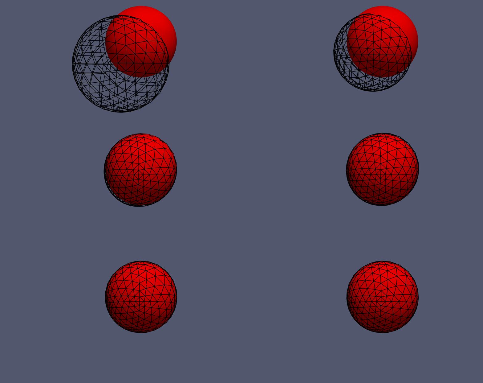
We can inspect the result by opening the file levelset_domain.pvd with ParaView. In the GIF below, we see that the domain (black grid) converges to the right shape (red ball).