Example 3: Kinetic energy dissipation in a pipe

In this example, we show how to minimize the shape functional

\[\mathcal{J}(\Omega) = \int_\Omega \nu \nabla \mathbf{u} : \nabla \mathbf{u} \,\mathrm{d}\mathbf{x}\,,\]

where \(\mathbf{u}:\mathbb{R}^d\to\mathbb{R^d}\,, d = 2,3,\) is the velocity of an incompressible fluid and \(\nu\) is the fluid viscosity. The fluid velocity \(\mathbf{u}\) and the fluid pressure \(p:\mathbb{R}^d\to\mathbb{R}\) satisfy the incompressible Navier-Stokes equations

\begin{align*} -\nu \Delta \mathbf{u} + \mathbf{u} \nabla \mathbf{u} + \nabla p &= 0 & \text{in } \Omega\,,\\ \operatorname{div} \mathbf{u} &= 0& \text{in } \Omega\,,\\ \mathbf{u} &= \mathbf{g} &\text{on } \partial\Omega\setminus \Gamma\,,\\ p\mathbf{n} - \nu \nabla u\cdot \mathbf{n} & = 0 &\text{on } \Gamma\,. \end{align*}

Here, \(\mathbf{g}\) is given by a Poiseuille flow at the inlet and is zero on the walls of the pipe. The letter \(\Gamma\) denotes the outlet.

In addition to the PDE-contstraint, we enforce a volume constraint: the volume of the optimized domain should be equal to the volume of the initial domain.

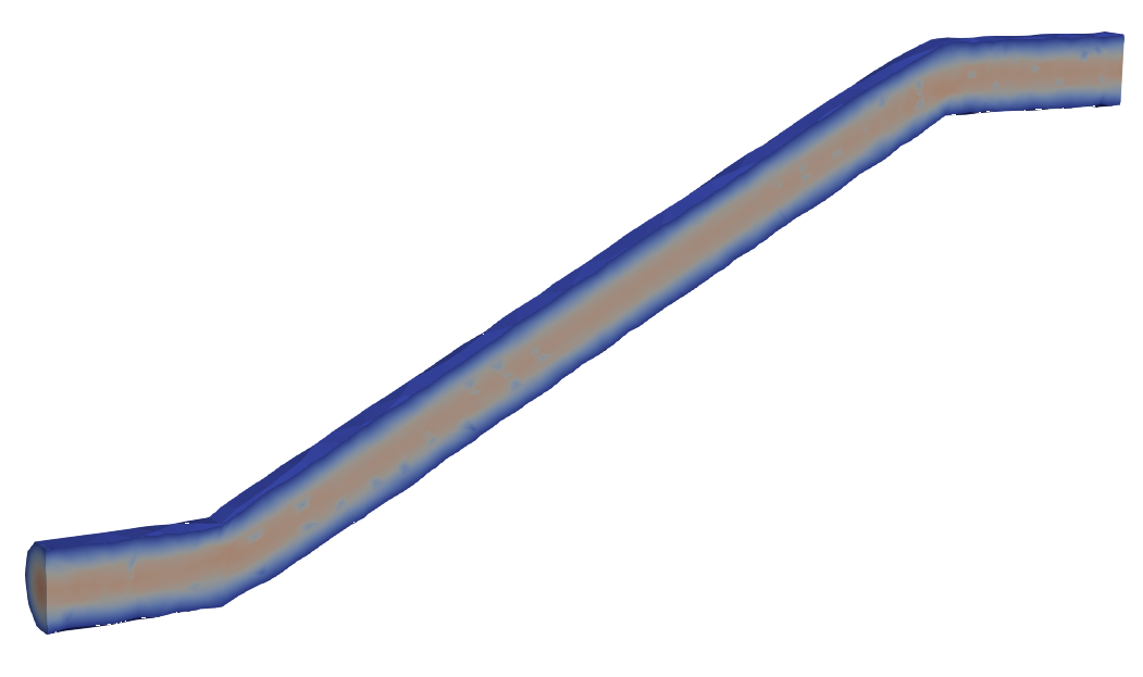
Initial domain

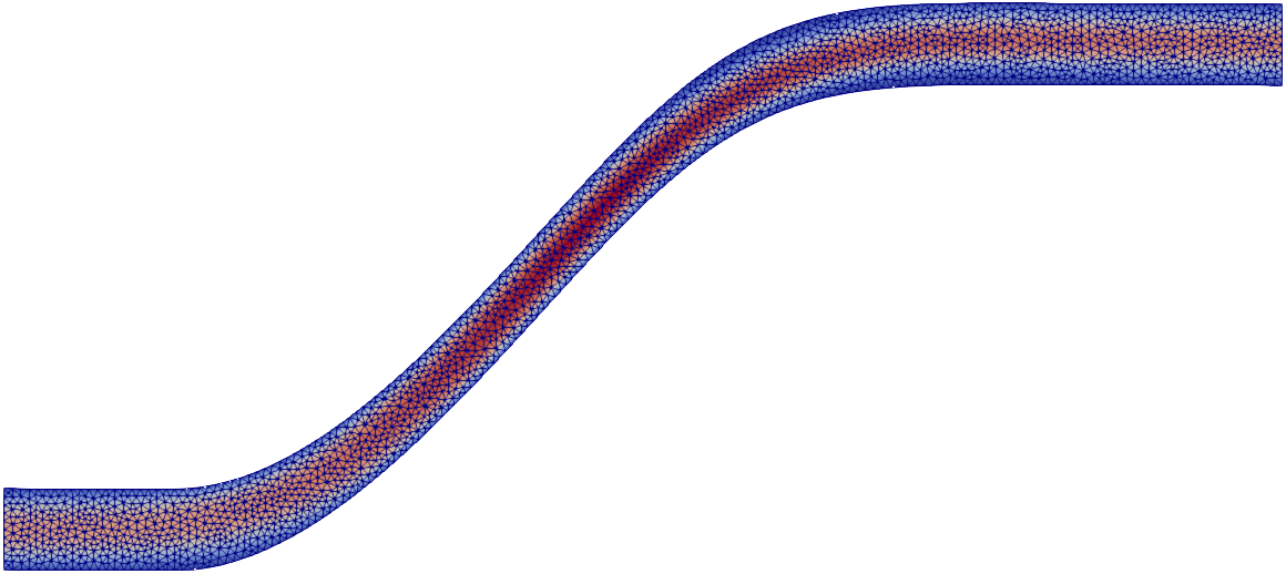
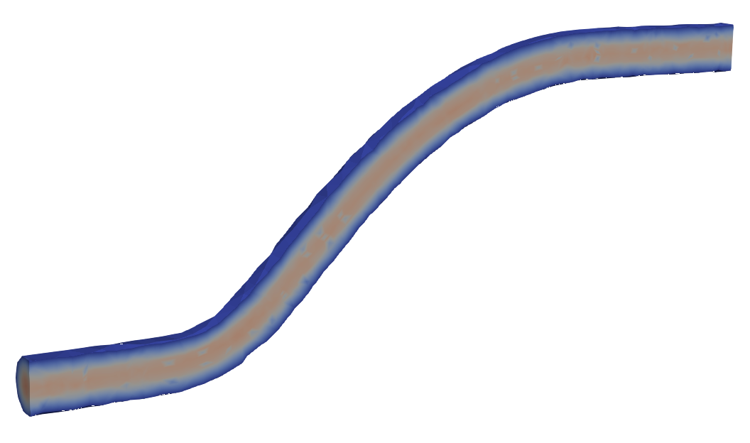
Initial pipe design in 2D (with mesh) and 3D, and magnitude of fluid velocity.

For the 2D-example, the geometry of the initial domain is described in the following gmsh script (this has been tested with gmsh v4.1.2).

h = 1.; //width
H = 5.; //height

//lower points
Point(1) = { 0, 0, 0, 1.};
Point(2) = { 2, 0, 0, 1.}; //first spline point
Point(3) = { 4, 0, 0, 1.};
Point(4) = { 8, 6, 0, 1.};
Point(5) = {10, 6, 0, 1.};
Point(6) = {12, 6, 0, 1.}; //last spline point
Point(7) = {15, 6, 0, 1.};
//upper points
Point( 8) = {15, 7, 0, 1.};
Point( 9) = {12, 7, 0, 1.}; //first spline point
Point(10) = {10, 7, 0, 1.};
Point(11) = { 8, 7, 0, 1.};
Point(12) = { 4, 1, 0, 1.};
Point(13) = { 2, 1, 0, 1.}; //last spline point
Point(14) = { 0, 1, 0, 1.};

//edges
Line(1) = {1, 2};
BSpline(2) = {2, 3, 4, 5, 6};
Line(3) = {6, 7};
Line(4) = {7, 8};
Line(5) = {8, 9};
BSpline(6) = {9, 10, 11, 12, 13};
Line(7) = {13, 14};
Line(8) = {14,  1};

//boundary and physical curves
Curve Loop(9) = {1, 2, 3, 4, 5, 6, 7, 8};
Physical Curve("Inflow", 10) = {8};
Physical Curve("Outflow", 11) = {4};
Physical Curve("WallFixed", 12) = {1, 3, 5, 7};
Physical Curve("WallFree", 13) = {2, 6};


//domain and physical surface
Plane Surface(1) = {9};
Physical Surface("Pipe", 2) = {1};

The mesh can be generated typing gmsh -2 -clscale 0.1 -format msh2 -o pipe.msh pipe2d.geo in the terminal.

For the 3D-example, the geometry of the initial domain is described in the following gmsh script.

// Gmsh project created on Tue Jan 22 11:40:52 2019
SetFactory("OpenCASCADE");
Circle(1) = {0, 0, 0, 0.5, 0, 2*Pi};
Line Loop(2) = {1};
Plane Surface(1) = {2};
Point( 5) = {0, 0.0,  0.00, 1.0};
Point( 6) = {0, 0.0,  2.00, 1.0}; //first spline point
Point( 7) = {0, 0.0,  3.00, 1.0};
Point( 8) = {0, 0.0,  4.00, 1.0};
Point( 9) = {0, 0.2,  4.75, 1.0};
Point(10) = {0, 5.0,  6.00, 1.0};
Point(11) = {0, 5.0, 10.00, 1.0};
Point(12) = {0, 5.0, 12.00, 1.0}; //last spline point
Point(13) = {0, 5.0, 15.00, 1.0};

Bezier(10) = {6, 7, 8, 9, 10, 11, 12};
Line(15) = {5, 6};
Line(16) = {12, 13};
Wire(1) = {15, 10, 16};
Extrude { Surface{1}; } Using Wire {1}
Delete{ Surface{1}; }

// When using fancy commands like "extrude", it is not quite obvious
// what the numbering of the generated lines, surfaces and volumes is
// going to be. To figure this out, we open the .geo file in the gmsh
// gui and use the Tools -> Visibility menu to find the numbers for
// each entity.

Physical Surface("Inflow", 10) = {2};
Physical Surface("Outflow", 11) = {6};
Physical Surface("WallFixed", 12) = {3, 5};
Physical Surface("WallFree", 13) = {4};
//Physical Surface("Inflow") = {2};
//Physical Surface("Outflow") = {6};
//Physical Surface("WallFixed") = {3, 5};
//Physical Surface("WallFree") = {4};
Physical Volume("PhysVol") = {1};

The mesh can be generated typing gmsh -3 -clscale 0.2 -format msh2 -o pipe.msh pipe3d.geo in the terminal (this has been tested with gmsh v4.1.2).

Implementing the PDE constraint

We implement the boundary value problem that acts as PDE constraint in a python module named PDEconstraint_pipe.py. In the code, we highlight the lines which characterize the weak formulation of this boundary value problem.

Note

The Dirichlet boundary data \(\mathbf{g}\) depends on the dimension \(d\) (see Lines 36-42)

import firedrake as fd
from fireshape import PdeConstraint


class NavierStokesSolver(PdeConstraint):
    """Incompressible Navier-Stokes as PDE constraint."""

    def __init__(self, mesh_m, viscosity):
        super().__init__()
        self.mesh_m = mesh_m
        self.failed_to_solve = False  # when self.solver.solve() fail

        # Setup problem, Taylor-Hood finite elements
        self.V = fd.VectorFunctionSpace(self.mesh_m, "CG", 2) \
            * fd.FunctionSpace(self.mesh_m, "CG", 1)

        # Preallocate solution variables for state equation
        self.solution = fd.Function(self.V, name="State")
        self.testfunction = fd.TestFunction(self.V)

        # Define viscosity parameter
        self.viscosity = viscosity

        # Weak form of incompressible Navier-Stokes equations
        z = self.solution
        u, p = fd.split(z)
        test = self.testfunction
        v, q = fd.split(test)
        nu = self.viscosity  # shorten notation
        self.F = nu*fd.inner(fd.grad(u), fd.grad(v))*fd.dx - p*fd.div(v)*fd.dx\
            + fd.inner(fd.dot(fd.grad(u), u), v)*fd.dx + fd.div(u)*q*fd.dx

        # Dirichlet Boundary conditions
        X = fd.SpatialCoordinate(self.mesh_m)
        dim = self.mesh_m.topological_dimension()
        if dim == 2:
            uin = 4 * fd.as_vector([(1-X[1])*X[1], 0])
        elif dim == 3:
            rsq = X[0]**2+X[1]**2  # squared radius = 0.5**2 = 1/4
            uin = fd.as_vector([0, 0, 1-4*rsq])
        else:
            raise NotImplementedError
        self.bcs = [fd.DirichletBC(self.V.sub(0), 0., [12, 13]),
                    fd.DirichletBC(self.V.sub(0), uin, [10])]

        # PDE-solver parameters
        self.nsp = None
        self.params = {
            "snes_max_it": 10, "mat_type": "aij", "pc_type": "lu",
            "pc_factor_mat_solver_type": "superlu_dist",
            # "snes_monitor": None, "ksp_monitor": None,
        }

    def solve(self):
        super().solve()
        self.failed_to_solve = False
        u_old = self.solution.copy(deepcopy=True)
        try:
            fd.solve(self.F == 0, self.solution, bcs=self.bcs,
                     solver_parameters=self.params)
        except fd.ConvergenceError:
            self.failed_to_solve = True
            self.solution.assign(u_old)


if __name__ == "__main__":
    mesh = fd.Mesh("pipe.msh")
    if mesh.topological_dimension() == 2:  # in 2D
        viscosity = fd.Constant(1./400.)
    elif mesh.topological_dimension() == 3:  # in 3D
        viscosity = fd.Constant(1/10.)  # simpler problem in 3D
    else:
        raise NotImplementedError
    e = NavierStokesSolver(mesh, viscosity)
    e.solve()
    print(e.failed_to_solve)
    out = fd.File("temp_PDEConstrained_u.pvd")
    out.write(e.solution.split()[0])

Note

The Navier-Stokes solver may fail to converge if too big an optimization step occurs in the optimization process. To address this issue, we use a trust-region algorithm as optimization solver, and we make the functional \(\mathcal{J}\) return NaN whenever the state solver fails. This way, the trust-region method will notice that there is no improvement if the state solver fails and will thus reduce the trust-region radius.

If the trust-region radius is too large, the algorithm may try to evaluate the objective functional on a domain that is not feasible. In this case, the PDE-solver fails, the domain is rejected, and the trust-region radius is reduced.

Implementing the shape functional

We implement the shape functional \(\mathcal{J}\) in a python file named objective_pipe.py. In the code, we highlight the lines which characterize \(\mathcal{J}\).

import firedrake as fd
from fireshape import ShapeObjective
from PDEconstraint_pipe import NavierStokesSolver
import numpy as np


class PipeObjective(ShapeObjective):
    """L2 tracking functional for Poisson problem."""

    def __init__(self, pde_solver: NavierStokesSolver, *args, **kwargs):
        super().__init__(*args, **kwargs)
        self.pde_solver = pde_solver

    def value_form(self):
        """Evaluate misfit functional."""
        nu = self.pde_solver.viscosity

        if self.pde_solver.failed_to_solve:  # return NaNs if state solve fails
            return np.nan * fd.dx(self.pde_solver.mesh_m)
        else:
            z = self.pde_solver.solution
            u, p = fd.split(z)
            return nu * fd.inner(fd.grad(u), fd.grad(u)) * fd.dx

Setting up and solving the problem

We set up the problem in the script main_pipe.py.

To set up the problem, we need to:

• load the mesh of the initial guess (Line 9),

• choose the discretization of the control (Line 10, Lagrangian finite elements of degree 1),

• choose the metric of the control space (Line 11, \(H^1\)-seminorm with homogeneous Dirichlet boundary conditions on fixed boundaries),

• initialize the PDE contraint on the physical mesh mesh_m (Line 15-21), choosing different viscosity parameters depending on the physical dimension dim

• specify to save the function \(\mathbf{u}\) after each iteration in the file solution/u.pvd by setting the function cb appropriately (Lines 24-28),

• initialize the shape functional (Line 31), and the reduced shape functional (Line 32),

• add a regularization term to improve the mesh quality in the updated domains (Lines 35-36),

• specify the volume equality constraint (Lines 39-42)

• create a ROL optimization prolem (Lines 45-58), and solve it (Line 60). Note that the volume equality constraint is imposed in Line 58.

import firedrake as fd
import fireshape as fs
import fireshape.zoo as fsz
import ROL
from PDEconstraint_pipe import NavierStokesSolver
from objective_pipe import PipeObjective

# setup problem
mesh = fd.Mesh("pipe.msh")
Q = fs.FeControlSpace(mesh)
inner = fs.LaplaceInnerProduct(Q, fixed_bids=[10, 11, 12])
q = fs.ControlVector(Q, inner)

# setup PDE constraint
if mesh.topological_dimension() == 2:  # in 2D
    viscosity = fd.Constant(1./400.)
elif mesh.topological_dimension() == 3:  # in 3D
    viscosity = fd.Constant(1/10.)  # simpler problem in 3D
else:
    raise NotImplementedError
e = NavierStokesSolver(Q.mesh_m, viscosity)

# save state variable evolution in file u2.pvd or u3.pvd
if mesh.topological_dimension() == 2:  # in 2D
    out = fd.File("solution/u2D.pvd")
elif mesh.topological_dimension() == 3:  # in 3D
    out = fd.File("solution/u3D.pvd")


def cb():
    return out.write(e.solution.split()[0])


# create PDEconstrained objective functional
J_ = PipeObjective(e, Q, cb=cb)
J = fs.ReducedObjective(J_, e)

# add regularization to improve mesh quality
Jq = fsz.MoYoSpectralConstraint(10, fd.Constant(0.5), Q)
J = J + Jq

# Set up volume constraint
vol = fsz.VolumeFunctional(Q)
initial_vol = vol.value(q, None)
econ = fs.EqualityConstraint([vol], target_value=[initial_vol])
emul = ROL.StdVector(1)

# ROL parameters
params_dict = {
    'General': {'Print Verbosity': 0,  # set to 1 to understand output
                'Secant': {'Type': 'Limited-Memory BFGS',
                           'Maximum Storage': 10}},
    'Step': {'Type': 'Augmented Lagrangian',
             'Augmented Lagrangian':
             {'Subproblem Step Type': 'Trust Region',
              'Print Intermediate Optimization History': False,
              'Subproblem Iteration Limit': 10}},
    'Status Test': {'Gradient Tolerance': 1e-2,
                    'Step Tolerance': 1e-2,
                    'Constraint Tolerance': 1e-1,
                    'Iteration Limit': 10}}
params = ROL.ParameterList(params_dict, "Parameters")
problem = ROL.OptimizationProblem(J, q, econ=econ, emul=emul)
solver = ROL.OptimizationSolver(problem, params)
solver.solve()

Note

This problem can also be solved using Bsplines to discretize the control. For instance, one could replace Line 10-11 with

bbox = [(1.5, 12.), (0, 6.)]
orders = [4, 4]
levels = [4, 3]
Q = fs.BsplineControlSpace(mesh, bbox, orders, levels, boundary_regularities=[2, 0])
inner = fs.H1InnerProduct(Q)

In this case, the control is discretized using tensorized cubic (order = [4, 4]) Bsplines (roughly \(2^4\) in the \(x\)-direction \(\times\, 2^3\) in the \(y\)-direction; levels = [4, 3]). These Bsplines lie in the box with lower left corner \((1.5, 0)\) and upper right corner \((12., 6.)\) (bbox = [(1.5, 12.), (0, 6.)]). With boundary_regularities = [2, 0] we prescribe that the transformation vanishes for \(x=1.5\) and \(x=12\) with \(C^1\)-regularity, but it does not necessarily vanish for \(y=0\) and \(y=6\). In light of this, we do not need to specify fixed_bids in the inner product.

Using Bsplines to discretize the control leads to similar results.

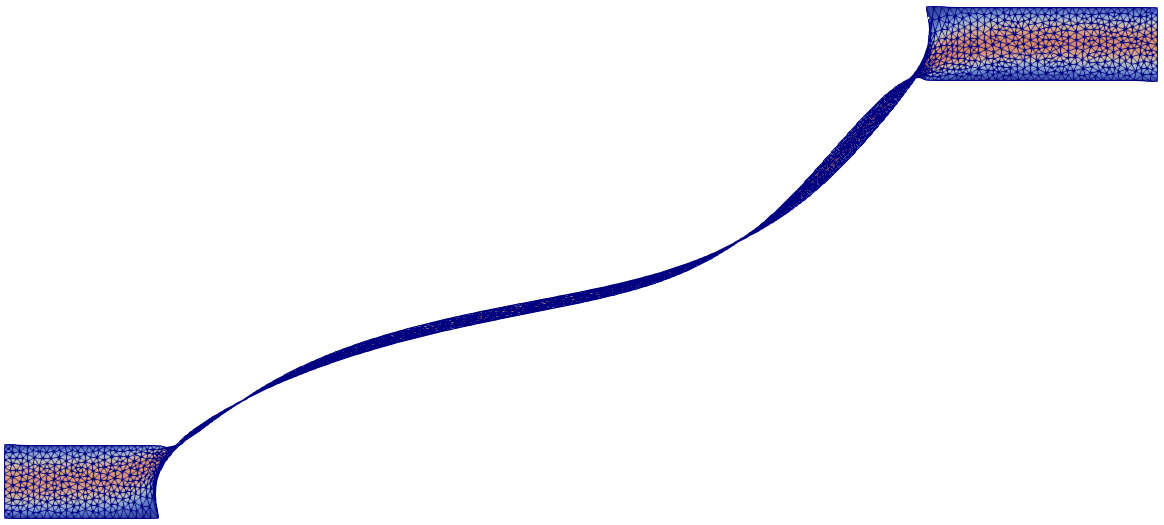
Result

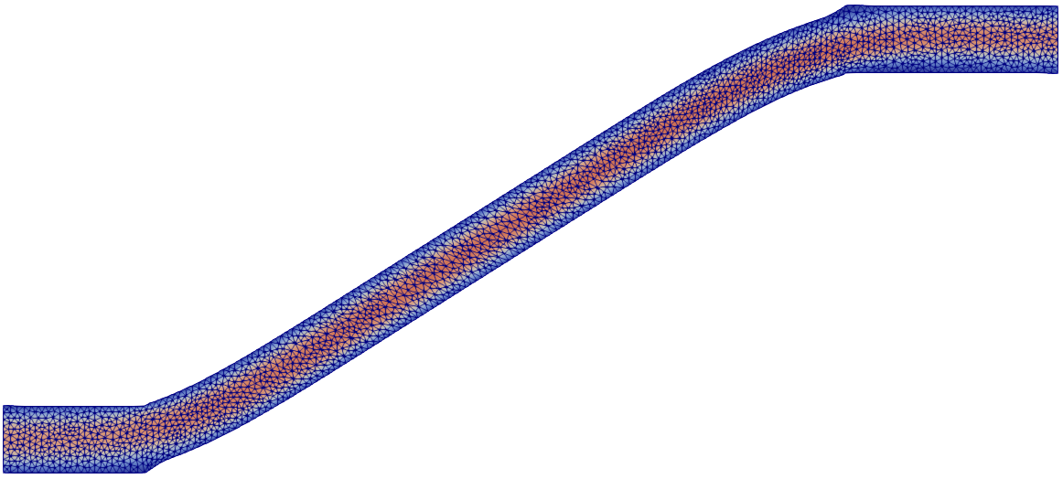
Optimized pipe design in 2D (left) and 3D (right).

For the 2D-example, typing python3 main_pipe.py in the terminal returns:

Augmented Lagrangian Solver
Subproblem Solver: Trust Region
  iter  fval           cnorm          gLnorm         snorm          penalty   feasTol   optTol    #fval   #grad   #cval   subIter
  0     4.390787e-01   0.000000e+00   4.690997e-01                  1.00e+01  1.26e-01  1.00e-02
  1     2.823114e-01   6.377197e-01   7.192107e-02   9.086354e-01   1.00e+02  1.26e-01  1.00e-01  15      11      22      10
  2     3.266521e-01   9.002146e-03   2.942106e-01   4.741487e-01   1.00e+02  7.94e-02  1.00e-03  23      15      32      5
  3     3.256262e-01   3.716964e-05   9.015756e-02   7.546472e-02   1.00e+02  5.01e-02  1.00e-04  36      25      53      10
  4     3.251405e-01   6.469895e-06   5.961345e-02   4.412538e-02   1.00e+02  3.16e-02  1.00e-04  49      35      74      10
  5     3.249782e-01   4.207885e-04   6.196224e-02   6.207929e-02   1.00e+02  2.00e-02  1.00e-04  62      45      95      10
  6     3.248956e-01   1.972863e-05   8.589613e-03   9.381617e-03   1.00e+02  1.26e-02  1.00e-04  75      55      116     10
Optimization Terminated with Status: Converged

Note

To store the terminal output in a txt file, use the bash command python3 main_pipe.py >> output.txt.

We can inspect the result by opening the file u.pvd with ParaView. We see that the difference between the volume of the initial guess and of the retrieved optimized design is roughly \(2\cdot 10^{-5}\).

For the 3D-example, typing python3 main_pipe.py in the terminal returns:

Augmented Lagrangian Solver
Subproblem Solver: Trust Region
  iter  fval           cnorm          gLnorm         snorm          penalty   feasTol   optTol    #fval   #grad   #cval   subIter
  0     1.211321e+01   0.000000e+00   1.000000e+00                  1.50e+01  1.00e-01  1.00e-02
  1     8.681223e+00   1.932438e+00   1.998650e-01   1.058693e+00   1.50e+02  8.72e-02  6.65e-02  15      13      24      10
  2     1.111633e+01   2.419067e-02   3.687839e-01   1.333067e+00   1.50e+02  5.28e-02  4.42e-04  23      19      36      5
  3     1.114521e+01   1.079619e-03   3.528500e-01   1.243047e-01   1.50e+02  3.20e-02  1.00e-04  36      29      57      10
  4     1.113536e+01   7.521605e-04   6.820438e-02   1.229308e-01   1.50e+02  1.94e-02  1.00e-04  49      39      78      10
  5     1.113373e+01   5.221684e-04   1.130481e-01   9.808759e-02   1.50e+02  1.17e-02  1.00e-04  62      49      99      10
  6     1.113360e+01   3.785105e-04   5.083579e-02   7.107051e-02   1.50e+02  7.11e-03  1.00e-04  75      59      120     10
  7     1.113168e+01   2.478858e-04   8.290102e-02   4.790457e-02   1.50e+02  4.30e-03  1.00e-04  88      69      141     10
  8     1.113127e+01   6.115143e-05   6.973287e-02   4.889087e-02   1.50e+02  2.61e-03  1.00e-04  101     79      162     10
  9     1.113080e+01   1.956210e-04   3.754803e-02   3.813478e-02   1.50e+02  1.58e-03  1.00e-04  114     89      183     10
  10    1.112986e+01   5.181766e-06   3.406590e-02   2.990831e-02   1.50e+02  1.00e-03  1.00e-04  127     99      204     10
Optimization Terminated with Status: Iteration Limit Exceeded

We can inspect the result by opening the file u.pvd with ParaView. We see that the difference between the volume of the initial guess and of the retrieved optimized design is roughly \(5\cdot 10^{-6}\).